Shalini's Knowledge Share

Little bit about shapefiles;

One way of storing Geographic data is using a shape file format. Shape file format is created by ESRI which consists of vector data. ESRI Technical Documentation describes the shapefile as something that stress nontopological geometry and attribute information for spatial features in a data set. Geometry for a feature is stored as a shape consisting a set of vector coordinates.

Shapefiles can support point, line and area features.

This article will describe how I have processed a shape file consisting of area features. Area features are represented as polygons.

An ESRI shapefile consists of 3 main types of files;

1. main file (.shp)
2. index file (shx)
3. dBase file (.dbf)

I’m not going to write about the specifics of each file as it is described well in the below technical document;

http://www.esri.com/library/whitepapers/pdfs/shapefile.pdf

Azure Databricks

If you have not gone through the above technical document, in short what we have is;

1. The main file (.shp) consists of the polygons.
2. dBase (.dbf) file consists of the actual data related to the census.

This article will discuss in length of how I have used Azure Databricks to process the shape files published in ABS (Australian Bureau of Statistics).

According to the ABS, the structure of the Australian Statistical Geography is divided into 7 levels of hierarchies:

1. Australia
2. States and Territories
3. Statistical Area Level 4 (SA4)
4. Statistical Area Level 3 (SA3) – Councils
5. Statistical Area Level 2 (SA2) – ex Suburb levels
6. Statistical Area Level 1 (SA1) –
7. Mesh blocks

SA1 is an aggregation of mesh blocks. SA2 is an aggregation of SA1 and so on. Examples – several suburbs make up of a council. (in other words, SA3 is an aggregation of SA2)

Reading shape files:

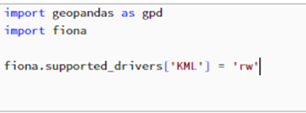
1. I have used GeoPandas library to process the shape files. Hence run pip install geopandas
2. Since I need to convert the final output to KML, I’m asking python to support KML drivers.

1. Read the shapefile. I store the shapefiles in a blob storage

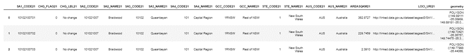
In the above few processes, I have read the shape file into a geopanda dataframe. (A dataframe is a data structure that organizes data into a 2D table of rows and columns, much like an SQL table having a similar structure called Schema. This can span into multiple computers making big data analytics possible.)

Also note that I have read the SA1 shapefile, which means it different polygons for each small geographical area.

Below is 3 rows of the data frame. You have the data and the polygons under geometry column.

Although the ABS website provides separate shape files for all the 4 statistical areas, I used only the SA1 shapefile as it contains data for all Statistical areas and States and Territories.

Please also note, that if you are directly trying to filter the polygons of SA1 by SA2, 3 or 4, this means you are using a larger data set. For this reason, best way to go is aggregating or dissolving of polygons.

Dissolving of Polygons:

If you extract the kml file for this, you will notice, the number of polygons have reduced as SA2 covers a larger area compared to SA1

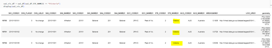
Filtering Polygons:

You can also filter the Polygons based on a column(s). In the below example, I have filtered by State = Victoria.

Plot the maps:

Below maps is plotted based on the SA1 and SA4 data frames respectively. Note the difference in number of polygons.

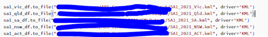
Converting to KML file:

Below I’m using the KML driver to convert each dataframe (I have created separate dataframe for each state, as we wont be using KML files for all states at once. This will improve the performance at the front end)